← (ne03) The Electric Field 電場 →

PreAmble: Newton (1643 - 1727) & Faraday (1791 - 1867)

• Electric field (Previous Lecture)
• Particle has (q, m) and a {observables}
• Newton: a = m / ΣF   (F includes contact and non-contact forces)
• ΣF = F_contact + Fg + Fe + ...
• Faraday: For long range forces, better to think of fields as intermediary (like talk-air-ear). On earth surface: ΣF = F_contact + m g + q E + ...

Key Points: Electric (Gravitational) Fields

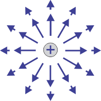
Point Charges & Symmetry

For Macroscopic objects we need to (Σ) or ∫ over all q (electric) or m (gravity). Generally this is done numerically. But there are a few simple cases...

4 Simple Cases
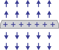
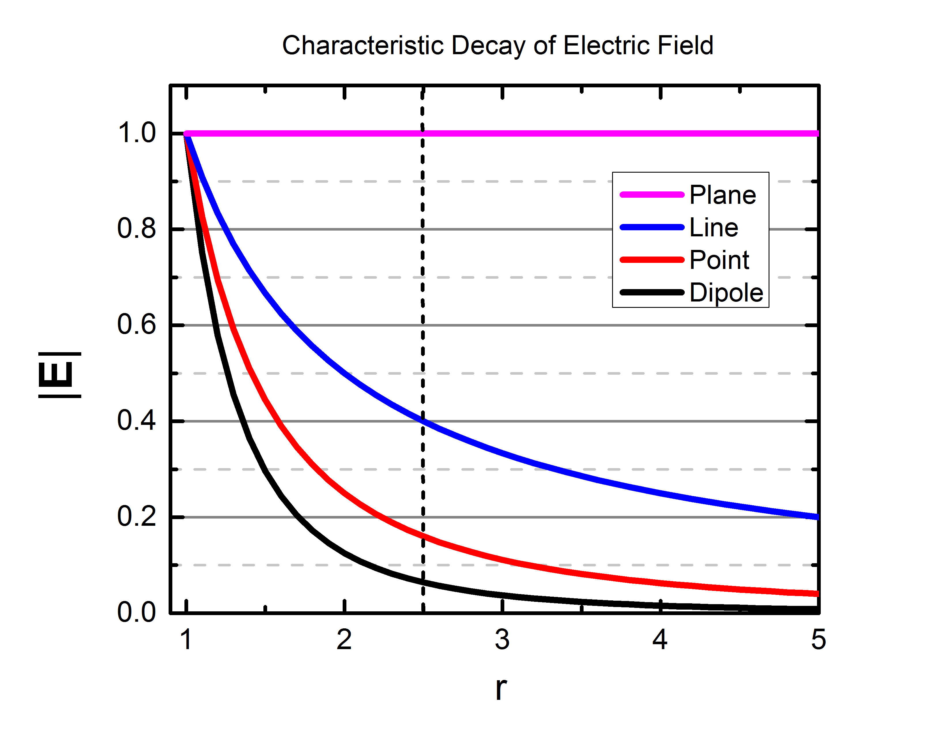
$$ \mathbf E_{point} $$	$$ \mathbf E_{line,\infty} $$	$$ \mathbf E_{plane,\infty} \, $$	$$ \mathbf E_{sphere} $$
$$ q \, [C] $$	$$ \lambda \, [C m^{-1}] $$	$$ \eta \, [C m^{-2} ] $$	$$ Q \, [C] \, $$
$$ = {1 \over {4 \pi \epsilon_o}} \, \color{fuchsia} {q \over r^2} \, { \mathbf r \over r } $$	$$ = {1 \over {4 \pi \epsilon_o}} \, \color{fuchsia}{2 \lambda \over r} \, { \mathbf r \over r } $$	$$ = {1 \over {4 \pi \epsilon_o}} \, \color{fuchsia}{2 \pi\eta } \, { \mathbf z \over z } $$	$$ = \mathbf E_{point} $$

Dipoles

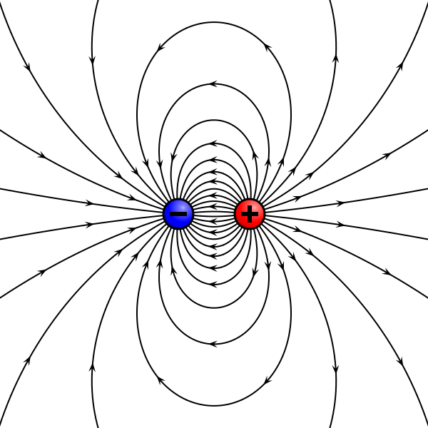
	$$ \mathbf p = |q| \, \mathbf {s} \, $$
	$$ \mathbf E_{dipole,axis} $$	$$ \mathbf E_{dipole,plane} $$
	$$ = {1 \over {4 \pi \epsilon_o}} \, \color{fuchsia} {2 \mathbf p \over r^3} $$	$$ = {1 \over {4 \pi \epsilon_o}} \, \color{fuchsia} { \mathbf p \over r^3} $$

(Observable) Acceleration: Linear & Angular

$$ \mathbf a = { q \over m_e} \mathbf E + { m_g \over m_e} \mathbf G $$

$$ \mathbf \alpha = {{\mathbf \tau} \over {I}} = {{\mathbf p \times \mathbf E} \over I} $$

Powerpoint & Kahoot

1 Review by Kahoot

2 Electric Dipole: intro then ppt23-31 to 42

3 Continous Charge Distributions - Line of Charge 43-54

4 Continue Charge Distributions - Rings/Disks/Planes/Spheres 55-63

5 Parallel Plate Capacitor 64-73

6,7 Motion in Electric Fields 74-100

Charged particle
Dipole (no charge, ΣFe=0 but the field does something....)